Example 1
We use a Langevin Generator tuned to generate the trajectories of a lysozyme molecule in water. After generating a significant amount of trajectories, we analyze the statistics of them and observe the classical scaling laws of the Langevin theory to explain Brownian Motion.
- The example is structured as follows:
Note
You can access the script of this example on the yupi examples repository.
1. Setup dependencies
Import all the dependencies:
import matplotlib.pyplot as plt
import numpy as np

from yupi.generators import LangevinGenerator
from yupi.graphics import plot_2d
from yupi.stats.kurtosis import KurtosisStat
from yupi.stats.msd import MsdTimeAvgStat
from yupi.stats.speed import SpeedStat
from yupi.stats.turning_angles import TurningAngleStat
from yupi.stats.vacf import VacfTimeAvgStat
2. Definition of parameters
First, we define some physical constants:
N0 = 6.02e23      # Avogadro's constant [1/mol]
k = 1.38e-23      # Boltzmann's constant [J/mol.K]
T = 300           # absolute temperature [K]
eta = 1.002e-3    # water viscosity [Pa.s]
M = 14.1          # lysozyme molar mass [kg/mol] [1]
d1 = 90e-10       # semi-major axis [m] [2]
d2 = 18e-10       # semi-minor axis [m] [2]
Then, we can indirectly measure quantities that are related with the physical model:
m = M / N0                   # mass of one molecule
a = np.sqrt(d1/2 * d2/2)     # radius of the molecule
alpha = 6 * np.pi * eta * a  # Stoke's coefficient
v_eq = np.sqrt(k * T / m)    # equilibrium thermal velocity
tau = m / alpha              # relaxation time
Next, we compute actual statistical model parameters for the Langevin Generator:
gamma = 1 / tau                   # drag parameter
sigma = np.sqrt(2 / tau) * v_eq   # scale parameter of noise pdf
Finally, we define general simulation parameters:
dim = 2                # trajectory dimension
N = 1000               # number of trajectories
dt = 1e-1 * tau        # time step
tt = 50 * tau          # total time
3. Generating trajectories
Once we have all the parameters required to tune the Langevin Generator, we just need to instantiate the class and generate the Trajectories:
lg = LangevinGenerator(T=tt, dim=dim, dt=dt, gamma=gamma, sigma=sigma, seed=0)
trajs = lg.generate(N)
4. Data analysis and plots
Let us initialize an empty figure for plot all the results:
plt.figure(figsize=(9,5))
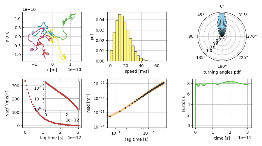
Plot spacial trajectories
plot_2d(trajs[:5], legend=False, ax=plt.subplot(231), show=False)
Plot speed histogram
SpeedStat(trajs).plot(bins=20, ax=plt.subplot(232), show=False)
Plot turning angles
TurningAngleStat(trajs).plot(
   bins=60, ax=plt.subplot(233, projection="polar"), show=False
)
Plot Velocity autocorrelation function
VacfTimeAvgStat(trajs, lag=50).plot(ax=plt.subplot(234), show=False)
Plot Mean Square Displacement
MsdTimeAvgStat(trajs, lag=50).plot(ax=plt.subplot(235), show=False)
Plot Kurtosis
KurtosisStat(trajs).plot(ax=plt.subplot(236), show=False)
Generate plot
plt.tight_layout()
plt.show()