Example 4
Tracking an intruder while penetrating a granular material in a quasi 2D enviroment. Code and multimedia resources are available here.
The work carried out by [1] studied penetration of an intruder inside a granular material, focusing on the influence of a wall on the trajectory of the intruder. The authors tested different configurations and observed specific phenomena during the penetration process (e.g., repulsion and rotation), as well as their dependence on the initial distance of the intruder from the wall.
In this example, we provide a script that extracts the trajectory of the intruder from one of the videos used to produce the results of the original paper. Moreover, we include details to generate a plot closely resembling the one presented in the paper [1].
- The example is structured as follows:
Note
You can access the script of this example on the yupi examples repository.
1. Setup dependencies
Import all the dependencies:
from numpy import pi
from yupi.graphics import plot_2d
from yupi.tracking.algorithms import ColorMatching
from yupi.tracking.trackers import ROI, ObjectTracker, TrackingScenario
from yupi.tracking.undistorters import RemapUndistorter
from yupi.transformations import rotate_2d
Set up the path to multimedia resources:
video_path = 'resources/videos/Diaz2020.MP4'
camera_file = 'resources/cameras/gph3+.npz'
2. Tracking tracking objects
Since the camera used for this application introduced a considerable spherical distortion, we need to create an instance of an Undistorter to correct it:
undistorter = RemapUndistorter(camera_file)
The variable camera_file contains the path to a .npz file with the matrix of calibration for the specific camera configuration, more details on how to produce it can be found in here.
Then, we initialize two trackers, one for each marker of the intruder:
algorithm1 = ColorMatching((70,40,20), (160,80,20)) # BGR
cyan = ObjectTracker('center marker', algorithm1, ROI((50, 50)))

algorithm2 = ColorMatching((30,20, 50), (95, 45,120))
magenta = ObjectTracker('border marker', algorithm2,  ROI((30, 50)))
Now, we will create the TrackingScenario with the trackers and also the Undistorter.
scenario = TrackingScenario([cyan, magenta],
                         undistorter=undistorter)
Then, we track the video using the configured scenario providing the scaling factor (pix_per_m) and the frame to start the processing:
retval, tl = scenario.track(video_path, pix_per_m=2826, start_frame=200)
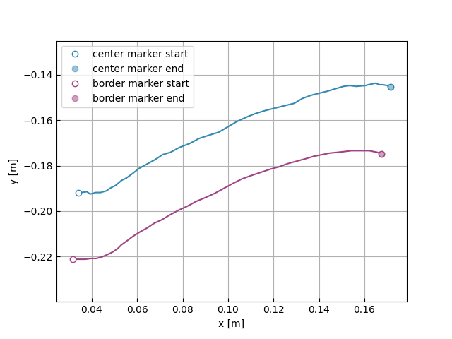
plot_2d(tl)
3. Computation of the variables
We can improve the visualization, by applying some transformations to the tracked trajectories. First, we can rotate them 90 degrees to better illustrate the effect of gravity:
rotate_2d(tl[0], -pi / 2)
rotate_2d(tl[1], -pi / 2)
Next, we update the coordinate system to place it at the initial position of the center of the intruder:
off = tl[0].r[0]
tl[1] -= off
tl[0] -= off
4. Results
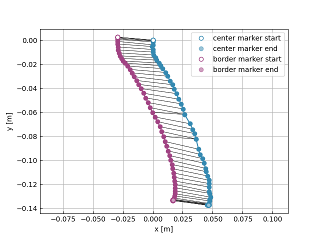
Now, we can produce a plot quite similar to the one of the original paper [1]:
plot_2d(tl, line_style='-o', connected=True)