Example 6
A comparison of different tracking methods over the same input video where the camera is fixed at a constant distance from the plane where an ant moves. Code and multimedia resources are available here.
In the work of Frayle-Pérez et. al [1], the authors studied the capabilities of different image processing algorithms that can be used for image segmentation and tracking of the motion of insects under controlled environments. In this section, we illustrate a comparison of a subset of these algorithms and evaluate them using one of the videos from the original paper.
- The example is structured as follows:
Note
You can access the script of this example on the yupi examples repository.
1. Setup dependencies
Import all the dependencies:
import cv2
from yupi.graphics import plot_2d
from yupi.tracking import (
   ROI,
   BackgroundEstimator,
   BackgroundSubtraction,
   ColorMatching,
   FrameDifferencing,
   ObjectTracker,
   OpticalFlow,
   TemplateMatching,
   TrackingScenario,
)
Set up the path to multimedia resources:
video_path = 'resources/videos/Frayle2017.mp4'
template_file = 'resources/templates/ant_small.png'
2. Creation of the tracking objects
First, we create an empty list to add all the trackers. Each tracker is associated with a tracking algorithm so we can evaluate the differences in the tracking process performed by each algorithm.
trackers = []
The first algorithm we will add is ColorMatching. It only requires the user to specify the range of colors that will considered by the algorithm as the ones belonging to the object. The range of colors can be indicated in different color spaces, by default BGR.
algorithm = ColorMatching((0,0,0), (150,150,150))
trackers.append( ObjectTracker('Ant (ColorMatching)', algorithm, ROI((50, 50))) )
In the case of FrameDifferencing, we specify the threshold in pixel intensity difference among two consecutive frames to be considered part of the tracked object.
algorithm = FrameDifferencing(frame_diff_threshold=5)
trackers.append( ObjectTracker('Ant (FrameDifferencing)', algorithm, ROI((50, 50))) )
BackgroundSubtraction algorithm requires a picture that contains only the background of the scene. However, if there is none available, it is possible to estimate it from a video using a BackgroundEstimator. Then, we specify the background_threshold that indicates the the minimum difference in pixel intensity among a frame and the background to be considered part of the moving object.
background = BackgroundEstimator.from_video(video_path, 20)
algorithm = BackgroundSubtraction(background, background_threshold=5)
trackers.append( ObjectTracker('Ant (BackgroundSubtraction)', algorithm, ROI((50, 50))) )
For the case of TemplateMatching algorithm, a template image containing a typical sample of the object being tracked must be provided. Then, it will compute the point in a frame in which the correlation between the template and the region of the frame is maximum.
template = cv2.imread(template_file)
algorithm = TemplateMatching(template, threshold=0.7)
trackers.append( ObjectTracker('Ant (TemplateMatching)', algorithm, ROI((50, 50))) )
OpticalFlow algorithm computes a dense optical flow among the current frame and the i-th previous frame, specified by the parameter buffer_size. If the magnitude of the flow is above a certain threshold it will be considered as part of the moving object.
algorithm = OpticalFlow(threshold=0.3, buffer_size=3)
trackers.append( ObjectTracker('Ant (OpticalFlow)', algorithm, ROI((50, 50))) )
3. Results
Once all the trackers are collected in a list, we can create a TrackingScenario:
scenario = TrackingScenario(trackers)
and track the video using the configured scenario. The track method will process the video pointed by video_path, using the additional settings we provide. In this case we are using a scale factor of 1020 pixels per meter. We must initialize the ROI of each tracker manually, unless we stated it differently while creating each of the ROI instances of the trackers.
retval, tl = scenario.track(video_path, pix_per_m=1024)
After the tracking process finishes we will have a list of Trajectory objects
in the variable tl. We can plot them together to evaluate the consistency
of all methods.
plot_2d(tl)
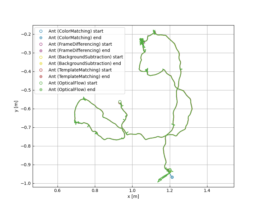
It is easy to see that the estimated trajectories are very consistent with each other despite the differences on the tracking methods. It is also important to realize that the differences in the very last part of the track are due the escape of the object being tracked from the scene. In those cases, each method does its own estimation of the likely next position.