Example 2
A model framework of a diffusion process with fluctuating diffusivity is presented. A Brownian but non-Gaussian diffusion by means of a coupled set of stochastic differential equations is predicted. Position is described by an overdamped Langevin equation and the diffusion coefficient as the square of an Ornstein-Uhlenbeck process.
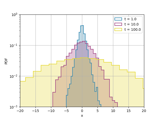
The example is focused in computing the probability density function for displacements at different time instants for the case of a one-dimensional process, as shown analitically by Chechkin et al. in [1] and discussed in [2].
- The example is structured as follows:
Note
You can access the script of this example on the yupi examples repository.
1. Setup dependencies
Import all the dependencies:
import numpy as np
from yupi.stats import collect
from yupi.graphics import plot_hists
from yupi.generators import DiffDiffGenerator
2. Definition of parameters
Simulation parameters:
T = 1000   # Total time of the simulation
N = 5000   # Number of trajectories
dt = .1    # Time step
3. Generating trajectories
Once we have all the parameters required, we just need to instantiate the class and generate the Trajectories:
dd = DiffDiffGenerator(T=T, dt=dt, seed=0)
trajs = dd.generate(N)
4. Data analysis and plots
Definition of time instants:
time_instants = np.array([1.0, 10.0, 100.0])
Let us obtain the position of all the trajectories in the key time instants:
r = [collect_at_time(trajs, time=t, func=lambda r: r.x) for t in time_instants]
Then, we can plot the results:
plot_hists(
   r,
   bins=30,
   density=True,
   labels=[f"t = {t}" for t in time_instants],
   xlabel="x",
   ylabel="PDF",
   legend=True,
   grid=True,
   yscale="log",
   ylim=(1e-3, 1),
   xlim=(-20, 20),
   filled=True,
)